Introduction
COordinate Rotation DIgital Computer (CORDIC) is an efficient iterative algorithm that uses rotations to compute some elementary functions. The algorithm is based on applying a sequence of rotations that only require additions, subtractions and bit shifts. Here I will present the principles of how the algorithm works, followed by how it is implemented to finally evaluate its accuracy for different bit-lengths.
Algorithm Intuition
Let’s start by giving an intuition of how the algorithm works.
Let a unitary vector form a counter-clockwise angle of \(\theta\) with the \(\begin{bmatrix}1\\0\end{bmatrix}\) vector:
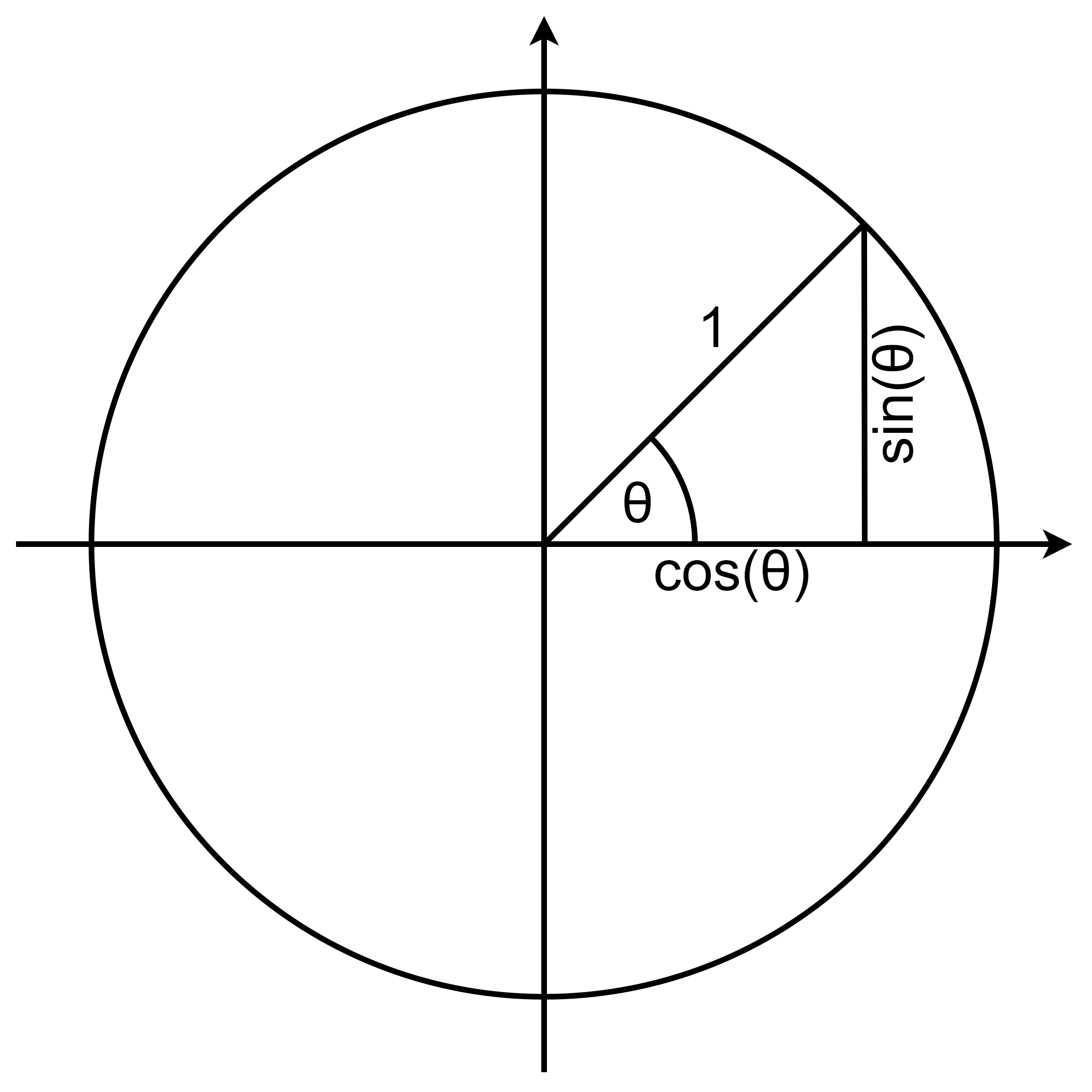
The \(\begin{bmatrix}\cos(\theta)\\ \sin(\theta)\end{bmatrix}\) vector can be expressed as a rotation of the \(\begin{bmatrix}1\\0\end{bmatrix}\) vector by an angle of \(\theta\):
\begin{align*}
\begin{bmatrix}\cos(\theta)\\ \sin(\theta)\end{bmatrix}
=
R(\theta)
\begin{bmatrix}1\\0\end{bmatrix}
\end{align*}
Where \(R(\theta)\) is the rotation matrix:
\begin{align*}
R(\theta) =
\begin{bmatrix}
\cos(\theta) &-\sin(\theta) \\
\sin(\theta) & \cos(\theta)
\end{bmatrix}
\end{align*}
An important property of the rotation operations is that:
\begin{align*}
\theta &= \alpha + \beta \\
\Rightarrow
R(\theta) &= R(\alpha) R(\beta)\\
\end{align*}
Now to compute \(\sin(\theta)\) and \(\cos(\theta)\), \(R(\theta)\) has to be decomposed into a sequence of precomputed rotation matrices:
\begin{align*}
\theta =& \theta_0 + \theta_1 \dotsi + \theta_n\\
\begin{bmatrix}\cos(\theta)\\ \sin(\theta)\end{bmatrix}
=&
R(\theta_0)R(\theta_1) \dotsi R(\theta_n)
\begin{bmatrix}1\\0\end{bmatrix}
\end{align*}
And that is the essence of how CORDIC works.
Algorithm Implementation
As shown previously, the computation of the sine and cosine can be reduced to a multiplication of precomputed matrices, which themself require addition, subtraction and multiplication of scalars. Of these three operations, multiplications are the most FPGA resource expensive, but through clever equation manipulation they can be eliminated:
\begin{align*}
R(\theta_i)
&=
\begin{bmatrix}
\cos(\theta_i) & -\sin(\theta_i) \\
\sin(\theta_i) & \cos(\theta_i)
\end{bmatrix} \\
&=
\cos(\theta_i)
\begin{bmatrix}
1 & -\frac{\sin(\theta_i)}{\cos(\theta_i)} \\
\frac{\sin(\theta_i)}{\cos(\theta_i)} & 1
\end{bmatrix} \\
&=
\cos(\theta_i)
\begin{bmatrix}
1 & -\tan(\theta_i) \\
\tan(\theta_i) & 1
\end{bmatrix}
\end{align*}
At this point the matrix-vector multiplication lost two multiplication operations, but the scalar multiplication appears to defeat the matrix multiplication reduction. Soon we will see that we can get rid of the \(\cos(\theta_i)\) multiplication, but before that we will make the matrix multiplication even simpler. To do this, \(\theta\) needs to be decomposed into a sequence of the following angles:
\begin{align*}
\theta_i = \arctan(2^{-i})
\end{align*}
Which turns the rotational matrices into:
\begin{align*}
R(\pm \theta_i)
&=
\cos(\theta_i)
\begin{bmatrix}
1 & \mp (2^{-i}) \\
\pm (2^{-i}) & 1
\end{bmatrix}
\end{align*}
Now the matrix multiplication contains one addition, one subtraction and two divisions by a power of 2 (which is just a right bit shift).
The algorithm finally turns into:
\begin{align*}
s_i &\in \{-1, 1\} \\ \\
\theta &= s_0 \theta_0 + s_1 \theta_1 + \dotsi + s_n \theta_n \\ \\
\Rightarrow
\begin{bmatrix}
\cos(\theta) \\ \sin(\theta)
\end{bmatrix}
&=
R(s_0 \theta_0)R(s_1 \theta_1) \dotsi R(s_n \theta_n)
\begin{bmatrix}
1 \\ 0
\end{bmatrix} \\
&=
\cos(\theta_0)
\begin{bmatrix}
1 & -s_0 \\
s_0 & 1
\end{bmatrix}
\cos(\theta_1)
\begin{bmatrix}
1 & -s_1 2^{-1} \\
s_1 2^{-1} & 1
\end{bmatrix}
\dotsi
\cos(\theta_n)
\begin{bmatrix}
1 & -s_n 2^{-n} \\
s_n 2^{-n} & 1
\end{bmatrix}
\begin{bmatrix}
1 \\ 0
\end{bmatrix} \\
&=
\begin{bmatrix}
1 & -s_0 \\
s_0 & 1
\end{bmatrix}
\begin{bmatrix}
1 & -s_1 2^{-1} \\
s_1 2^{-1} & 1
\end{bmatrix}
\dotsi
\begin{bmatrix}
1 & -s_n 2^{-n} \\
s_n 2^{-n} & 1
\end{bmatrix}
\prod_{i=0}^{n} \cos(\theta_i)
\begin{bmatrix}
1 \\ 0
\end{bmatrix} \\
\end{align*}
As it can be seen \(\prod_{i=0}^{n} \cos(\theta_i) \begin{bmatrix} 1 \\ 0 \end{bmatrix}\) is constant, so it can be precomputed. In this way the computation of sine and cosine can be decomposed into a sequence of additions, subtractions and divisions by powers of 2 (which can be implemented as right shifts).
The way to compute \(s_i\) is relatively simple:
\begin{align*}
s_i =
\begin{cases}
1,& \quad \text{if} \ \ (i = 0 \ \land \ \theta < 0) \ \lor \ (i > 0 \ \land \ \theta > \sum_{j=0}^{i-1} s_j \theta_j) \\
-1,& \quad \text{otherwise}
\end{cases}
\end{align*}
As it is the algorithm is constrained to \(\theta\) in the range of approximately \(-\pi/2\) to \(+pi/2\) (when setting all \(s_i\) variables to either -1 or 1).
To solve this, depending on the region where the \(\begin{bmatrix}\cos(\theta)\\ \sin(\theta)\end{bmatrix}\) vector falls, we can rotate a vector that is closer to it so that it does not need to be rotated more than \(\pm \pi/2\).
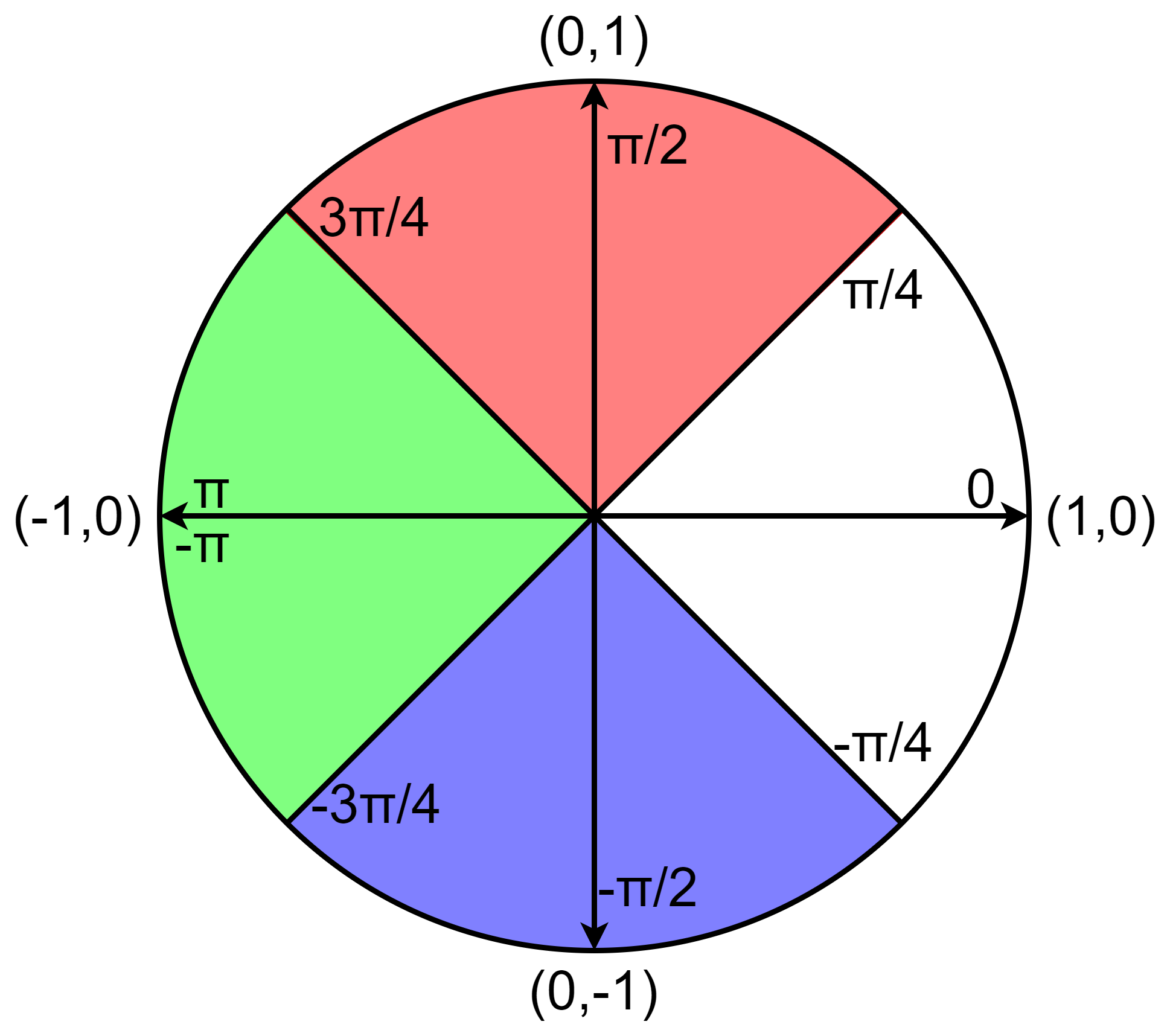
\begin{align*}
\begin{bmatrix}
\cos(\theta) \\ \sin(\theta)
\end{bmatrix}=
\begin{cases}
R(\theta) \begin{bmatrix}1 \\ 0\end{bmatrix}, & \quad \text{if} \ \ \theta \in [-\pi/4, \pi/4) \\
R(\theta – \pi/2) \begin{bmatrix}0 \\ 1\end{bmatrix}, & \quad \text{if} \ \ \theta \in [\pi/4, 3 \pi/4) \\
R(\theta + \pi/2) \begin{bmatrix}0 \\ -1\end{bmatrix}, & \quad \text{if} \ \ \theta \in [-3\pi/4, -\pi/2) \\
R(\theta + \pi) \begin{bmatrix}-1 \\ 0\end{bmatrix}, & \quad \text{if} \ \ \theta \in [-\pi, -3\pi/4) \ \lor \ \theta \in [3\pi/4, \pi)\\
\end{cases}
\end{align*}
All pieces of the piecewise function return the exact same value, but by choosing the proper piece, the rotations can be kept within the \(\pm \pi/2\) range. In this way it is possible to evaluate the sine and cosine functions for any \(\theta\).
Implementation Details
To evaluate the accuracy I implemented the algorithm in C++. Two fixed-point number formats for the input (angle) and the output (vector) were used. Turns were used as angle unit and two formats for its n-bit representation:
- 1 sign bit and n-1 bits for the powers \(2^{-1}, 2^{-2},…, 2^{-(n-1)}\).
- 1 sign bit and n-1 bits for the powers \(2^{-3}, 2^{-4},…, 2^{-(n+1)}\).
The reason to use two representations is that for a defined bit-length 2 extra bits can be gained after performing the first rotation. The first rotation always sets the \(2^{-1}\) and \(2^{-2}\) variable components to zero. So to increase the accuracy without increasing the bit-length, the variable is right-shifted 2 bits.
Accuracy Measurement
I evaluated the accuracy of the algorithm through the measurement of the error for every possible input angle for different bit-lengths. I covered inputs and outputs of bit-lengths from 4 bits to 32 bits. The statistics of the cosine and sine were evaluated together as a whole as they showed minimal differences.


Both diagrams show similar patterns, with the difference that the maximum absolute error diagram shows less regularity (probably caused by rounding artifacts).
For either the input or the output bit-lengths, increasing one without increasing the other has diminishing returns. For an equal input and output bit-length, increasing the input bit-length increases the accuracy very little, in contrast, increasing the output bit-length improves the accuracy much more.
Since the bit-lengths directly affect the FPGA resource requirements, finding the minimum required bit-length to achieve certain level of accuracy is important to optimize the resource usage. To aid in the selection of the right bit-length, I plotted the standard deviation of the error (bottom trace) and maximum absolute error (top trace) for different output bit-lengths minus input bit-lengths.
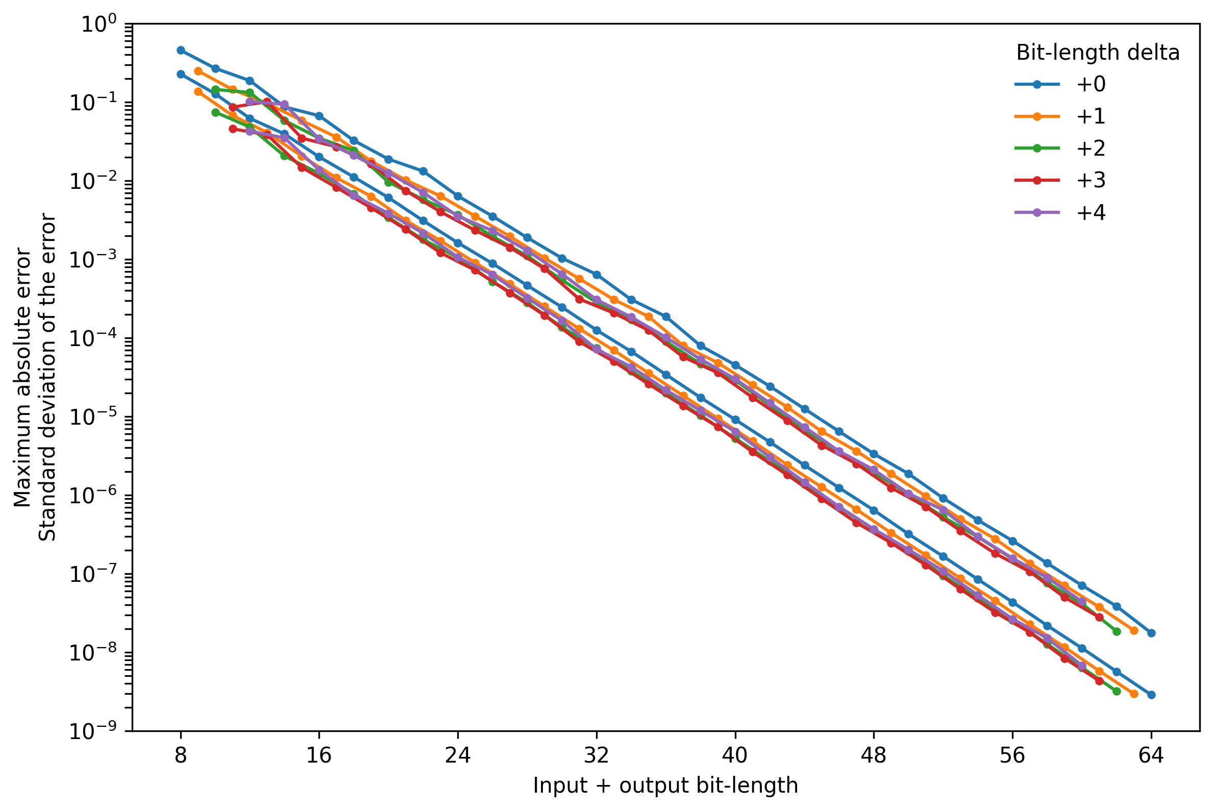
The traces show that almost for every total bit-length, the standard deviation of the error and the maximum error tend to be lowest when the output bit-length is 3 bits wider than the input bit-length.
To focus on the most relevant parts of the figure, I plotted the most accurate bit-length combination (in terms of standard deviation of the error and the maximum absolute error) for different total bit-lengths.
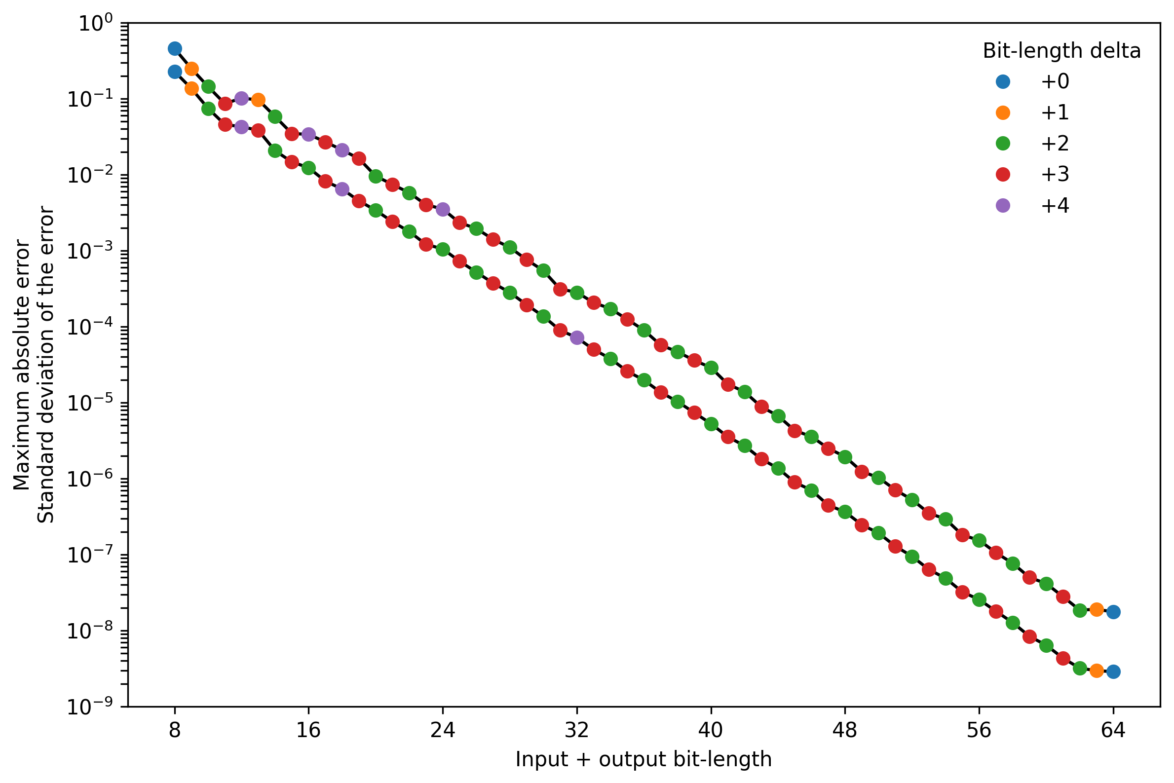
For most total bit-length combinations a delta of +2 and +3 produced the best results, with a few exceptions. Note that in both ends, the results are affected by the lack of evaluation of different bit-length combinations.
Conclusion
Too few bits to compute the sine and cosine using CORDIC can save FPGA resource, and allow faster clock speed, but also result in poor accuracy. Too many bits provide high accuracy but at high cost of FPGA resources and lower clock speed. So, what is the optimal bit-length? As usual, it depends on the application, but to answer that, it is necessary to know what accuracy can be achieved for different bit-lengths.
In this post I implement CORDIC in C++ and evaluated all possible inputs to compute statistics that can aid in the selection of the right input and output bit-length to achieve the desired level of accuracy.
The code is available on GitHub.